CS336 LLM from Scratch Lab1 writeup

概述

本系列为斯坦福 Stanford CS336 | Language Modeling from Scratch 课程的作业笔记。

该作业实现难度较大，实验文档正文就有足足 46 页，对算力也有相当大的需求。在此衷心感谢北京大学 Linux 俱乐部提供的算力资源和组织讨论平台。

本 lab 的相关代码仓库在此处，将其 clone 到本地即可。该实验使用 uv 管理环境，代码需要在 cs336_basics/ 中完成，test/ 中为测试点，在完成各个功能的时候需要同步实现 adapters.py 里面的接口。

这个 lab 需要实现：

• BPE 分词器；

• 从零开始实现一个 Transformer 模型（仅从 torch 里面的基本组件开始）；

  • 具体规则：

    We expect you to build these components from scratch. In particular, you may not use any definitions from torch.nn, torch.nn.functional, or torch.optim except for the following:

    • torch.nn.Parameter
    • Container classes in torch.nn (e.g., Module, ModuleList, Sequential, etc.)
    • The torch.optim.Optimizer base class

• CELoss 和 AdamW 优化器，以及余弦退火调度器；

• 训练循环相关逻辑，如 dataloader 以及 checkpoint 的读取/保存。

并且在 TinyStories 和 OpenWebText 两个数据集上进行大量对比/消融实验并分析结果。

我的实现放在 Cgfyufsygsm/CS336-assignment1-basics，供参考学习使用，请勿直接抄袭否则可能啥也没学到x

我花在这个 lab 上的时间粗略估计有至少 20+ 小时，想要尽可能自己实现所有内容是相当费劲的但也能让人对 LLM 的整个基本原理有更深入的理解。我也得以亲自搭一遍 Transformer 的完整结构并实现如 tokenizer 和 text generation 相关看似不核心但仍然很重要的逻辑。

目前我对 resource accounting 相关的计算的正确性仍然不是特别有把握，如有错误欢迎随时批评指正，不胜感激！

BPE Tokenizer

这部分是我认为这个 lab 最难的一部分，因为实现的方案完全由自己指定，而在处理大数据集的时候会不可避免地遇到性能问题。事实上这个 lab 最花时间的部分可能正是性能优化的部分。

Unicode Standard

(a) Unicode NULL 字符（U+0000）

(b) 转义字符 \x00，打印出来是不可见字符

© 出现在文本里面的话单纯是一个不可见字符

Unicode Encodings

(a) UTF-8 完全兼容 ASCII 字符，编码更紧凑，更省空间。UTF16/32 占用空间更多且引入大量高位 0 字节，浪费序列长度，增加冗余噪声。

(b) “你好”即可（包含非 ASCII 字符）。因为这个函数是逐字节解码的，但是一个 Unicode 字符在 UTF-8 表示下可能不止需要一个字节来表示，所以会出现问题。

© 0xC0 0x80 就不能被解码到任何 Unicode 字符上。

BPE Tokenizer

可以参考 Chen571428/cs336-assignment1-basics 的实现，其通过极致优化达到了极高的吞吐率。

这方面非常需要精细实现，好和差的实现可能效率差上几百上千倍，进而几乎无法处理 owt_train.txt 这种大达 11GB 的训练数据。几个比较关键的地方：

• pretokenization 的并行化
• BPE merge 的处理
• encoding 的并行化

完事了之后需要把这些训练数据都转成 numpy 格式的 token 序列并保存起来以供后文的 TransformerLM 使用。

一些我遇到的坑：

• merge 和 vocab 最好都把对应的字节串用某种方式（我用的是 GPT-2 使用的 encoding 方式）转成 UTF-8 可见字符然后以 json 格式输出，这样可以避免很多问题。
• 开过多的进程反而可能带来很多额外开销，得不偿失。
• 可以使用 rich 库来进行日志/进度条处理，效果很好。

Transformer LM Architecture

接下来的部分就比较简单一些了，虽然工作量不算小，但至少如果能过测试点则说明大概率没有什么问题。

Before we start

建议先仔细阅读文档 15-18 页对于 batched matmul 和 einops 的解释。虽然我的实现里没有使用 einops 但这种优雅的 self-documenting 实现还是值得学习的。

以及关于行向量还是列向量的处理，我的理解是线性代数里面使用列向量是更符合数学直觉（教科书里面一般也这样），但实现的时候使用行向量形式，一是因为 memory ordering 二是因为 batch 的存在，前者天然更适合 batch 化（当然如果使用 einsum 是不是好像就完全不用 care 了）。

Linear

实现一个不带 bias 的线性层。

class Linear(nn.Module):
    def __init__(self, in_features, out_features, device=None, dtype=None):
        super().__init__()
        self.in_features = in_features
        self.out_features = out_features
        self.weight = nn.Parameter(torch.empty((out_features, in_features), device=device, dtype=dtype))
        self._init_weight()

    def _init_weight(self):
        sigma = math.sqrt(2.0 / (self.in_features + self.out_features))
        nn.init.trunc_normal_(self.weight, std=sigma, a=-3*sigma, b=3*sigma)

    def forward(self, x):
        return x @ self.weight.T

几个细节：

• __init__ 里面要调用 super().__init__() 把 Module 给进行初始化。
• W 的维度应该是 (out, in)，这样对应着 $y = xW^\top$。这样是比存储 (in, out) 然后 $y = Wx$（线代里面常见写法）更合理的，其中一个原因就在于很多时候 $x$ 的维度是带 batch 的，比如 (B1, B2, in)，我们想获得 (B1, B2, out) 那自然是 $y = xW^\top$ 更合理。

Embedding

Transformer 的第一层，把整数 token 给映射到向量空间。相当于若输入是 (B, T, V)（这里的 $T$ 是序列长度，$V$ 是 vocab size）则应该输出 (B,T,D)（其中 $D$ 为每个 token 对应向量的维度）。

于是用一个 $V\times D$ 的矩阵来存参数，然后 forward 的时候用 token 值来索引就可以了：

class Embedding(nn.Module):
    def __init__(self, num_embeddings, embedding_dim, device=None, dtype=None):
        super().__init__()
        self.num_embeddings = num_embeddings
        self.embedding_dim = embedding_dim
        self.weight = nn.Parameter(torch.empty((num_embeddings, embedding_dim), device=device, dtype=dtype))
        self._init_weight()

    def _init_weight(self):
        nn.init.trunc_normal_(self.weight, std=1, a=-3, b=3) # 按照题目要求初始化

    def forward(self, x):
        return self.weight[x]

RMSNorm

现在广泛使用的 normalize 函数。对于 $a\in \mathbb{R}^{d_{\text{model}}}$，有

$$\text{RMSNorm}(a_i) = \frac{a_i}{\text{RMS}(a)}g_i$$

其中 $\text{RMS}(a) = \sqrt{\frac{1}{d_{\text{model}}}\sum_{i=1}^{d_{\text{model}}}a_i^2+\varepsilon}$，$g_i$ 为可学习的增益参数。

class RMSNorm(nn.Module):
    def __init__(self, d_model: int, eps: float = 1e-5, device=None, dtype=None):
        super().__init__()
        self.d_model = d_model
        self.eps = eps
        self.gain = nn.Parameter(torch.ones(d_model, device=device, dtype=dtype))

    def forward(self, x):
        in_dtype = x.dtype
        x = x.to(torch.float32) # 提示说要把输入的 x 给 upcast 到 torch.float32
        rms = torch.sqrt(torch.mean(x * x, dim=-1, keepdim=True) + self.eps)
        return ((x / rms) * self.gain).to(in_dtype)

SwiGLU

原始 Transformer 论文使用的 FFN 是 $W_2(\text{ReLU}(W_1x))$，现在常见的模型使用的是 Swish + 门控的方案。具体地，

$$\text{FFN}(x) = \text{SwiGLU}(x, W_1,W_2,W_3) = W_2(\text{SiLU}(W_1x) \odot W_3x)$$

注意到为了维持参数量一致，一般 $d_{\text{ff}} = \frac 83 d_{\text{model}}$。

def SiLU(x: torch.Tensor) -> torch.Tensor:
    """
    Given an input tensor `x`, return the SiLU activation applied elementwise.
    SiLU(x) = x * sigmoid(x)
    """
    return x * torch.sigmoid(x)

class SwiGLU(nn.Module):
    def __init__(self, d_model: int, d_ff: int, device=None, dtype=None):
        super().__init__()
        self.d_model = d_model
        self.d_ff = d_ff
        self.linear1 = Linear(d_model, d_ff, device=device, dtype=dtype)
        self.linear2 = Linear(d_ff, d_model, device=device, dtype=dtype)
        self.linear3 = Linear(d_model, d_ff, device=device, dtype=dtype)
    
    def forward(self, x: torch.Tensor) -> torch.Tensor:
        gate = SiLU(self.linear1(x))
        value = self.linear3(x)
        return self.linear2(gate * value)

RoPE

这是相对不太好写的一部分。

要做的事情是把一个 $d_k$ 维的向量的偶/奇维度配对，即 $0/1, 2/3, \cdots$ 配对，每一对施加旋转矩阵。第 $i$ 对子空间对应的频率为 $\omega_i = \Theta^{-2i/d_k}$，位置为 $p$ 时旋转角为 $\phi_{p,i} = p\cdot w_i$。

实现的时候，在 __init__ 里将 $\sin, \cos$ 信息给初始化缓存下来，免得 forward 的时候需要现算。

class RotaryPositionalEmbedding(nn.Module):
    def __init__(self, theta: float, d_k: int, max_seq_len: int, device=None):
        super().__init__()
        self.theta = theta
        self.d_k = d_k
        self.max_seq_len = max_seq_len

        assert(d_k % 2 == 0), "d_k must be even for Rotary Positional Embedding."
        half = d_k // 2
        k = torch.arange(half, device=device, dtype=torch.float32)
        inv_freq = torch.pow(theta, -2 * k / d_k)
        positions = torch.arange(max_seq_len, device=device, dtype=torch.float32)
        angle = positions[:, None] * inv_freq[None, :]
        cos_cached, sin_cached = torch.cos(angle), torch.sin(angle)
        self.register_buffer("cos_cached", cos_cached, persistent=False)
        self.register_buffer("sin_cached", sin_cached, persistent=False)

half 为子空间的对数，然后 k = torch.arange(half) 再 inv_freq = torch.pow(theta, -2 * k / d_k) 得到所有的 $d_k/2$ 个 $w_i$。然后 arange 出所有的 positions，对于 $\phi_{p,i}$ 直接广播出所有的 angle = positions[:, None] * inv_freq[None, :]，再求出相应的 sin_cached 和 cos_cached（维度均为 (max_seq_len, half)）。用 register_buffer 说明它不会被更新，persistent=False 说明不会被保存进 state_dict。

现在回忆一下对于 $(x_{\text{even}}, x_{\text{odd}})^\top$ 怎么做旋转：

$$\begin{pmatrix} \cos\theta& -\sin\theta\\ \sin\theta & \cos \theta \end{pmatrix}\begin{pmatrix} x_0\\x_1 \end{pmatrix} = \begin{pmatrix} x_0\cos\theta - x_1\sin\theta\\ x_0\sin\theta + x_1\cos\theta \end{pmatrix}$$

def forward(self, x: torch.Tensor, token_positions: torch.Tensor) -> torch.Tensor:
    x_pair = x.view(*x.shape[:-1], -1, 2)
    x_even = x_pair[..., 0]
    x_odd = x_pair[..., 1]
    cos_pos = getattr(self, "cos_cached")[token_positions]
    sin_pos = getattr(self, "sin_cached")[token_positions]
    x_even_rot = x_even * cos_pos - x_odd * sin_pos
    x_odd_rot = x_even * sin_pos + x_odd * cos_pos
    x_pair = torch.stack((x_even_rot, x_odd_rot), dim=-1)
    return x_pair.view(*x.shape[:-1], self.d_k)

注意这里的 token_positions 是给定的，不一定是完整的 $0,1,\cdots$。

首先用 view 把奇偶维度切开，此时的 x_even 和 x_odd 维度为 (..., seq_len, half)，token_positions 维度为 (..., seq_len)。

然后把对应位置的 cos 和 sin 给取出来，取出来的 cos_pos 维度为 (..., half)。然后就可以算新的 x_even 和 x_odd 了。最后 stack 起来再还原维度成 d_k 即可。

Scaled Dot-Product Attention

首先需要实现 softmax，需要在指定的维度进行 softmax，并把所有的项减去 $\max$ 以避免数值精度问题。

def softmax(x: torch.Tensor, dim: int) -> torch.Tensor:
    """
    Given an input tensor `x`, return the softmax applied along dimension `dim`.
    """
    exp_x = torch.exp(x - torch.max(x, dim=dim, keepdim=True).values)
    return exp_x / torch.sum(exp_x, dim=dim, keepdim=True)

然后实现

$$\text{Attention}(Q,K,V) = \text{softmax}\left(\frac{Q^\top K}{\sqrt{d_k}}\right)V$$

同时需要实现 masking。输入一个 (seq_len, seq_len) 的 mask，如果 mask[i, j] == False 说明 query $i$ 不应该注意到 key $j$。

首先明确一下这个函数的维度：

Args:
    Q (Float[Tensor, " ... queries d_k"]): Query tensor
    K (Float[Tensor, " ... keys d_k"]): Key tensor
    V (Float[Tensor, " ... values d_v"]): Values tensor
    mask (Bool[Tensor, " ... queries keys"] | None): Mask tensor
Returns:
    Float[Tensor, " ... queries d_v"]: Output of SDPA

实现的时候显然没法直接写 $Q^\top K$ 了，注意到我们需要的注意力分数维度应该是 (..., queries keys) 的（[i, j] 表示 how query $i$ attends to key $j$，且注意到 values 一般应当等于 keys）所以应当写成 score = q @ k.transpose(-2, -1)，即把 $K$ 的后两个维度转置一下。

完整代码如下，剩下的都不难，mask 可以直接在 softmax 之前把被 mask 住的地方赋 $-\inf$。

def scaled_dot_product_attention(q: torch.Tensor, k: torch.Tensor, v: torch.Tensor, mask: torch.Tensor | None = None):
    d_k = q.shape[-1]
    score = q @ k.transpose(-2, -1)
    scores = score / math.sqrt(d_k)
    if mask is not None:
        scores = scores.masked_fill(~mask, -torch.inf)
    attn = softmax(scores, dim=-1)
    return attn @ v

Causal Multi-Head Self-Attention

需要实现一个带 mask 的多头注意力机制并且使用 RoPE。

这里我的实现是将 RoPE 作为构造函数的参数直接传进来。

输入是 (..., seq_len, d_model) 的，要把 $x$ 拆成 $h$ 个并分给 $h$ 个注意力头。文档里面直接说了可以直接用 $W_Q,W_K\in \mathbb{R}^{hd_k\times d_{\text{model}}},W_V\in\mathbb{R}^{hd_v\times d_{\text{model}}}$ 来做。只要把 $h$ 也作为批量维度的一部分就可以直接用上面的函数来解决了。具体看代码注释。

class MultiheadSelfAttention(nn.Module):
    def __init__(self, d_model: int, num_heads: int, rope: RotaryPositionalEmbedding | None = None):
        super().__init__()
        self.d_model = d_model
        self.num_heads = num_heads
        assert d_model % num_heads == 0 # Ensure divisibility
        self.head_dim = d_model // num_heads

        self.W_Q = Linear(d_model, d_model)
        self.W_K = Linear(d_model, d_model)
        self.W_V = Linear(d_model, d_model)
        self.W_O = Linear(d_model, d_model)
        self.rope = rope


    def forward(self, x: torch.Tensor, token_positions: torch.Tensor | None = None) -> torch.Tensor:
        # x: (..., seq_len, d_model)
        q, k, v = self.W_Q(x), self.W_K(x), self.W_V(x) # (..., seq_len, d_model)
        q = q.view(*q.shape[:-1], self.num_heads, self.head_dim).transpose(-3, -2).contiguous() # (..., num_heads, seq_len, head_dim)
        # -2 is num_heads, -3 is seq_len, so need to transpose
        k = k.view(*k.shape[:-1], self.num_heads, self.head_dim).transpose(-3, -2).contiguous() # (..., num_heads, seq_len, head_dim)
        v = v.view(*v.shape[:-1], self.num_heads, self.head_dim).transpose(-3, -2).contiguous() # (..., num_heads, seq_len, head_dim)
        mask = torch.tril(torch.ones((x.shape[-2], x.shape[-2]), dtype=torch.bool, device=x.device)) # (seq_len, seq_len)
        # score[i, j] means how i attends to j, so we want to mask out j > i
        # so for j > i, we set mask[i, j] = False, thus lower triangular

        if self.rope is not None:
            if token_positions is None:
                token_positions = torch.arange(x.shape[-2], device=x.device)
            q = self.rope(q, token_positions)
            k = self.rope(k, token_positions)

        attn_output = scaled_dot_product_attention(q, k, v, mask=mask) # num_heads will be treated as batch dimension
        attn_output = attn_output.transpose(-3, -2).contiguous() # (..., seq_len, num_heads, head_dim)
        attn_output = attn_output.view(*attn_output.shape[:-2], self.d_model) # (..., seq_len, d_model)
        output = self.W_O(attn_output) # (..., seq_len, d_model)
        return output

Transformer

$$y = x + \text{MultiHeadSelfAttention}(\text{RMSNorm}(x))$$

实现一个 pre-norm 结构的 Transformer Block。没什么好说的直接套娃之前的就行了。

class TransformerBlock(nn.Module):
    def __init__(self, d_model: int, num_heads: int, d_ff: int, theta: float = 100000.0, max_seq_len: int = 2048):
        """
        d_model: int Dimensionality of the Transformer block inputs.
        num_heads: int Number of heads to use in multi-head self-attention.
        d_ff: int Dimensionality of the position-wise feed-forward inner layer.
        """
        super().__init__()
        self.norm1 = RMSNorm(d_model)
        rope = RotaryPositionalEmbedding(theta, d_model // num_heads, max_seq_len=max_seq_len)
        self.attn = MultiheadSelfAttention(d_model, num_heads, rope)
        self.norm2 = RMSNorm(d_model)
        self.ffn = SwiGLU(d_model, d_ff)

    def forward(self, x: torch.Tensor):
        y = x + self.attn(self.norm1(x))
        return y + self.ffn(self.norm2(y))

最后把他们都套起来：

class TransformerLM(nn.Module):
    def __init__(self, d_model: int, num_heads: int, d_ff: int, vocab_size: int, context_length: int, num_layers: int, rope_theta: float = 100000.0):
        super().__init__()
        self.token_embedding = Embedding(vocab_size, d_model)
        self.attention_blocks = nn.Sequential(*[TransformerBlock(
            d_model,
            num_heads,
            d_ff,
            theta=rope_theta,
            max_seq_len=context_length
        ) for _ in range(num_layers)])
        self.norm = RMSNorm(d_model)
        self.linear = Linear(d_model, vocab_size)
        # 注意这里没有说要 softmax，在 generate 的时候再说
        
    def forward(self, x: torch.Tensor):
        x = self.token_embedding(x)
        x = self.attention_blocks(x)
        x = self.norm(x)
        x = self.linear(x)
        return x

Resource accounting

统计参数量和 FLOPS。计算方法：对于 $A\in \mathbb{R}^{m\times n}, B\in \mathbb{R}^{n\times p}$，相乘需要 $2mnp$ 个 FLOPs。

• 对于 GPT-2 XL，如下参数：

  vocab_size: 50257
  context_length: 1024
  num_layers: 48
  d_model: 1600
  num_heads: 25
  d_ff: 6400

  可训练的参数数量：

  • embedding 和 output linear 各 $V\times d$
  • 对于每层 Transformer block：
    • $W_Q,W_K,W_V,W_O$ 有 $4d^2$
    • 这里的 $d_{\text{ff}}$ 似乎是 $4d$，就当他是传统 MLP 吧，两层线性层有 $2d\cdot d_{\text{ff}}$
    • 两个 RMSNorm 有 $2d$
  • output RMSNorm 有一个 $d$。

  所以一共是 $2Vd+N(4d^2+2dd_{\text{ff}}+2d)+d=2Vd+N(12d^2+2d)+d$$2Vd + N(4d^2 + 2d\cdot d_{ff} + 2d) + d = 2Vd+N(12d^2+2d)+d$，代入参数计算得到约 1.64B，float32 的话约 6.1GB

• 计算一次前向传播的 FLOPs

  设 context_length 为 $L$：

  • Q/K/V 投影：3 次 $(L\times d)\cdot(d\times d)$ → $6 L d^2$
  • O 投影：1 次 $(L\times d)\cdot (d\times d)$ → $2 L d^2$
  • 注意力分数：$QK^\top$ $(L\times d)\cdot (d\times L)$ → $2 L^2 d$
  • 注意力加权：$\text{Attn}\cdot V$ $(L\times L)\cdot (L\times d)$→ $2 L^2 d$
  • FFN：$2 L d d_{\text{ff}}\times 2$ → $4 L d d_{\text{ff}}$
  • 所以一层的是 $8Ld^2 + 4L^2d + 4Ldd_{ff} = 24Ld^2 + 4L^2d$
  • 输出线性：$(L\times d)\cdot (d\times V)$ → $2 L d V$

  所以是 $N(24Ld^2+4L^2d)+2LdV$ 代入得到约 3.51 TFLOPS

• 分析哪部分需要最多的 FLOPs

  FFN 占约 57.4%，最大；注意力投影约 28.7%；注意力分数/加权约 9.2%；输出线性约 4.7%。

• 假设 GPT‑2 small/medium/large 都是 d_ff=4*d_model，且 $L=1024, V=50257$。各组件 FLOPs 占比如下（占总 FLOPs）：

  模型	Attn proj	Attn inner	FFN	LM head
  GPT-2 small (12L, d=768, h=12)	19.88%	13.25%	39.76%	27.10%
  GPT-2 medium (24L, d=1024, h=16)	24.93%	12.47%	49.86%	12.75%
  GPT-2 large (36L, d=1280, h=20)	27.23%	10.89%	54.46%	7.42%
  GPT-2 XL (48L, d=1600, h=25)	28.71%	9.19%	57.41%	4.70%

  随着模型变大，$d^2$ 规模的项（投影、FFN）比重上升，$L^2 d$ 的注意力分数项和输出线性（$L~d~V$）比重下降；因此 FFN 占比越来越大，输出线性占比快速降低。

• GPT‑2 XL 把 $L$ 从 1024 提到 16384（16 倍），$L^2$ 项增长 256 倍，其余 $L$ 项增长 16 倍。总 FLOPs 从 3.51e12 变为 1.33e14，约 38.05 倍；注意力分数/加权项占比跃升到 约 61.81%，FFN 降到约 24.14%，投影约 12.07%，输出线性约 1.97%。

Training a Transformer LM

Cross-entropy Loss

Transformer 对于 (B, seq_len) 的 token 输入，输出的 logits 是 (B, seq_len, vocab_size) 的，相当于是“每个位置上的 next-token prediction”。那么监督信号自然是用输出的 logits 和真实的 target 做 cross-entropy loss。具体地来看就是文档里的

$$l_i = -\log \text{softmax}(o_i)[x_{i+1}] = -\log\frac{\exp(o_i[x_{i+1}])}{\sum_{a=1}^{\texttt{vocab\_size}}\exp(o_i[a])}$$

文档里说要考虑数值稳定性，避免不必要的 $\log$ 和 $\exp$，所以先让 $o$ 减去 $\max$，变成 $z$，再把上面的式子拆一下：

$$-\log\frac{\exp(o_i[x_{i+1}])}{\sum_{a=1}^{\texttt{vocab\_size}}\exp(o_i[a])} = \log\sum_{a=1}^{\texttt{vocab\_size}}\exp(z_i[a]) - z_i[x_{i+1}]$$

def CrossEntropyLoss(input: torch.Tensor, target: torch.Tensor):
    z = input - input.max(dim=-1, keepdim=True).values
    log_denom = torch.logsumexp(z, dim=-1, keepdim=True)
    z_true = z.gather(dim=-1, index=target.unsqueeze(-1)).squeeze(-1)
    loss = (-z_true + log_denom).mean()
    return loss

因为取 z_true 是想要 z[i, target_i] 所以这里需要用 gather。

The SGD Optimizer

文档让我们尝试调整 SGD 的 learning rate。发现 1e1 收敛过慢，1e2 正好，1e3 loss 直接爆炸了。

AdamW

实现是简单的，直接依葫芦画瓢就行：

class AdamW(torch.optim.Optimizer):
    def __init__(self, params, lr=1e-3, betas=(0.9, 0.999), eps=1e-8, weight_decay=0.01):
        if lr < 0.0:
            raise ValueError(f"Invalid learning rate: {lr}")
        if not 0.0 <= betas[0] < 1.0:
            raise ValueError(f"Invalid beta parameter at index 0: {betas[0]}")
        if not 0.0 <= betas[1] < 1.0:
            raise ValueError(f"Invalid beta parameter at index 1: {betas[1]}")
        if eps < 0.0:
            raise ValueError(f"Invalid epsilon value: {eps}")
        if weight_decay < 0.0:
            raise ValueError(f"Invalid weight_decay value: {weight_decay}")

        defaults = dict(lr=lr, betas=betas, eps=eps, weight_decay=weight_decay)
        super().__init__(params, defaults)
    
    def step(self, closure: Optional[Callable]=None):
        loss = None if closure is None else closure()
        for group in self.param_groups:
            lr = group["lr"]
            beta1, beta2 = group["betas"]
            eps = group["eps"]
            weight_decay = group["weight_decay"]

            for p in group["params"]:
                if p.grad is None:
                    continue
                grad = p.grad.data
                state = self.state[p]

                if len(state) == 0:
                    state["t"] = 0
                    state["m"] = torch.zeros_like(p.data)
                    state["v"] = torch.zeros_like(p.data)
                
                state["m"] = beta1 * state["m"] + (1 - beta1) * grad
                state["v"] = beta2 * state["v"] + (1 - beta2) * (grad ** 2)
                state["t"] += 1
                t = state["t"]
                alpha_t = lr * math.sqrt(1 - beta2 ** t) / (1 - beta1 ** t)
                p.data -= alpha_t * state["m"] / (torch.sqrt(state["v"]) + eps)
                p.data -= lr * weight_decay * p.data
        return loss

Resource accounting:

(a) 分析如下：

• 参数量见上，$P = 2Vd + N(12d^2+2d)+d$，占用显存 $M_{\text{param}} = 4P$ bytes
• 每个参数一个梯度，$M_{\text{grad}} = 4P$ bytes
• Adam 维护两个动量，$M_{\text{opt}} = 8P$ bytes
• Activations:
  • 每层 Transformer block:
    • RMSNorm $\times 2$：$2BLd$
    • QKV project：$3BLd$
    • $QK^\top$：$BhL^2$
    • softmax 输出：$BhL^2$
    • 加权求和输出： $BLd$
    • 最终投影：$BLd$
    • FFN：$BLd_{ff} + BLd_{ff} + BLd$
  • 所以 $A_{\text{layer}} = 16BLd+2BhL^2$
  • final RMSNorm：$BLd$
  • output logits：$BLV$
  • CELoss：$BLV$
  • 所以总共是 $A = N(16BLd+2BhL^2)+BLd+2BLV$
  • $M_{\text{act}} = 4A$ bytes
• 峰值显存为 $M_{\text{peak}} = 16P + 4A$ bytes

(b) 代入数据计算即可，解得 $B_{\max} = 3$

© $3B(L(24Ld^2+4L^2d)+2LdV) + \Theta(P)$

• Forward FLOPS：只考虑 matmul，则：$F_{\text{fwd}} = B(L(8Ld^2+4L^2d+4Ldd_{ff})+2LdV) = B(L(24Ld^2+4L^2d)+2LdV)$
• Backward FLOPS：近似两倍 $2F_{\text{fwd}}$ 以及一次逐元素 $F_{\text{adam}} = \Theta(P)$

(d) 每 step 的 FLOPS：$3\times 1024 \times (L(24Ld^2+4L^2d)+2LdV) \approx 1.08\times 10^{16}$，一共 $400$K 步，所以 $t = \frac{F_{\text{total}}}{19.5\times 50\%} = 4.419\times 10^8$ s，即 14 年（？）

Learning Rate Scheduling

文档里要求使用 LLaMA 的余弦退火。

即先 warm-up，然后 cosine，最后维持 min lr。

def lr_cosine_schedule(
    it: int,
    max_learning_rate: float,
    min_learning_rate: float,
    warmup_iters: int,
    cosine_cycle_iters: int,
):
    if it < warmup_iters:
        lr = it / warmup_iters * max_learning_rate
    elif it <= cosine_cycle_iters:
        lr = min_learning_rate + 0.5 * (max_learning_rate - min_learning_rate) * (1 + math.cos(math.pi * (it - warmup_iters) / (cosine_cycle_iters - warmup_iters)))
    else:
        lr = min_learning_rate
    return lr

Gradient Clipping

限制梯度的 L2-Norm 不要太大避免梯度爆炸：

def gradient_clipping(parameters: Iterable[torch.nn.Parameter], max_l2_norm: float):
    eps = 1e-6
    for p in parameters:
        if p.grad is None:
            continue
        param_norm = p.grad.data.norm(2)
        if param_norm > max_l2_norm:
            clip_coef = max_l2_norm / (param_norm + eps)
            p.grad.data.mul_(clip_coef)

Training Loop

DataLoader

根据文档的说法直接弄就行，相当于随机 sample batch_size 个 start 点，然后往后找 context_length 这么长的数据。一起返回就好了。

def get_batch(
    dataset: np.ndarray,
    batch_size: int,
    context_length: int,
    device: str,
) -> tuple[torch.Tensor, torch.Tensor]:
    """
    Sample language modeling batches from a 1D token ID array.

    Returns:
        Tuple of LongTensors (x, y) with shape (batch_size, context_length).
    """
    if dataset.ndim != 1:
        raise ValueError("dataset must be a 1D numpy array of token IDs")
    max_start = len(dataset) - context_length
    if max_start <= 0:
        raise ValueError("dataset length must be greater than context_length")

    starts = np.random.randint(0, max_start, size=batch_size)
    x_np = np.stack([dataset[i : i + context_length] for i in starts], axis=0)
    y_np = np.stack([dataset[i + 1 : i + context_length + 1] for i in starts], axis=0)

    x = torch.tensor(x_np, dtype=torch.long, device=device)
    y = torch.tensor(y_np, dtype=torch.long, device=device)
    return x, y

Checkpointing

利用好 torch 的 state_dict() 就可以了。

import torch
import os
import typing

def save_checkpoint(
    model: torch.nn.Module,
    optimizer: torch.optim.Optimizer,
    iteration: int,
    out: str | os.PathLike | typing.BinaryIO | typing.IO[bytes]
):
    state = {
        "model_state_dict": model.state_dict(),
        "optimizer_state_dict": optimizer.state_dict(),
        "iteration": iteration,
    }
    torch.save(state, out)

def load_checkpoint(
    src: str | os.PathLike | typing.BinaryIO | typing.IO[bytes],
    model: torch.nn.Module,
    optimizer: torch.optim.Optimizer
):
    state = torch.load(src)
    model.load_state_dict(state["model_state_dict"])
    optimizer.load_state_dict(state["optimizer_state_dict"])
    return state["iteration"]

Training Loop

这个每个人写的脚本都不尽相同，主要提几个点：

• 每个 it 的循环内，先用余弦退火算出 lr，然后设置 optimizer 里面的 lr；然后用之前写的 get_batch sample 出这一轮需要的 batch，调用 model(x) 算出 logits，再计算 loss；然后 loss.backward()，梯度裁剪，再 optimizer.step() 更新参数。
• 在合适的时候 log/保存 checkpoint 即可。
• 涉及到的参数可能巨多无比，需要想一下怎么管理参数。我的做法是用一个 config.py 来维护，然后可以在命令行里面传参进行覆盖。

Generating Text

我们生成文字的时候是自回归（autoregressive）式的生成，每次喂进去已有的序列，然后获得下一个 token 的概率分布并 sample 之。具体地即

$$\begin{aligned} P(x_{t+1}=i \mid x_{1,\cdots,t}) &= \frac{\exp(v_i)}{\sum_j \exp(v_j)}\\ v &= \text{TransformerLM}(x_{1,\cdots,t})_t\in\mathbb{R}^{\texttt{vocab\_size}} \end{aligned}$$

相当于，每次喂进去的是一个长度为 $\texttt{seq\_len}$ 的 token 序列，然后输出的是 $\texttt{seq\_len}\times\texttt{vocab\_size}$ 的 logits，我们取最后一行来预测下一个位置的 token。然后反复做这个过程，直到达到最大上下文长度或者遇到 $\texttt{<|endoftext|>}$。

具体地有两个参数可以设置，一个是温度 Temperature ($\tau$)，一个是 top-p sampling 的 $p$。前者是在 softmax 里面除以 $\tau$ 来控制模型生成文本的“集中程度”。当 $\tau\to 0$ 则更接近 one-hot 编码（强烈放大最大概率的 token），反之亦然。Top-p 又称为核心采样，将小概率的 token 进行截断，即令 $V(p)$ 为最小的能使 $\sum_{j\in V(p)} q_j\ge p$ 的 index 集合，其中 $q_j$ 为 temperature-scaled softmax 输出的概率分布，然后把概率调整为 $\frac{q_i}{\sum_{j\in V(p)} q_j}$（对于 $V(p)$ 中的），而把 $V(p)$ 外的全部设置成 $0$。

写一个 decoding.py：

import torch
from torch import Tensor

from cs336_basics.nn.util import softmax


def apply_temperature(logits: Tensor, temperature: float) -> Tensor:
    """
    Scale logits by temperature. Lower temperature sharpens the distribution.
    """
    if temperature <= 0:
        raise ValueError("temperature must be > 0 for scaling")
    return logits / temperature


def top_p_filter(logits: Tensor, top_p: float) -> Tensor:
    """
    Apply nucleus (top-p) filtering to logits.
    Keeps the smallest set of tokens whose cumulative probability >= top_p.
    """
    if top_p >= 1.0:
        return logits
    if top_p <= 0.0:
        top_idx = logits.argmax(dim=-1, keepdim=True)
        mask = torch.ones_like(logits, dtype=torch.bool)
        mask.scatter_(-1, top_idx, False)
        return logits.masked_fill(mask, -float("inf"))

    probs = softmax(logits, dim=-1)
    sorted_probs, sorted_idx = probs.sort(dim=-1, descending=True)
    cumulative = sorted_probs.cumsum(dim=-1)

    cutoff = cumulative > top_p
    cutoff[..., 1:] = cutoff[..., :-1].clone()
    cutoff[..., 0] = False

    mask = torch.zeros_like(cutoff).scatter(-1, sorted_idx, cutoff)
    return logits.masked_fill(mask, -float("inf"))


def sample_next_token(
    logits: Tensor,
    temperature: float = 1.0,
    top_p: float = 1.0,
    rng: torch.Generator | None = None,
) -> Tensor:
    """
    Sample token ids from logits (shape: [batch, vocab] or [vocab]).
    """
    squeeze_out = False
    if logits.dim() == 1:
        logits = logits.unsqueeze(0)
        squeeze_out = True

    if temperature <= 0:
        next_ids = logits.argmax(dim=-1)
        return next_ids.squeeze(0) if squeeze_out else next_ids

    scaled = apply_temperature(logits, temperature)
    filtered = top_p_filter(scaled, top_p)
    probs = softmax(filtered, dim=-1)
    next_ids = torch.multinomial(probs, num_samples=1, generator=rng).squeeze(-1)
    return next_ids.squeeze(0) if squeeze_out else next_ids


@torch.no_grad()
def generate_tokens(
    model: torch.nn.Module,
    prompt_ids: Tensor | list[int],
    max_new_tokens: int,
    eos_id: int | None = None,
    temperature: float = 1.0,
    top_p: float = 1.0,
    context_length: int | None = None,
    rng: torch.Generator | None = None,
) -> Tensor:
    """
    Autoregressively generate tokens from a prompt.
    """
    device = next(model.parameters()).device
    if torch.is_tensor(prompt_ids):
        prompt = prompt_ids.to(device=device, dtype=torch.long)
    else:
        prompt = torch.tensor(prompt_ids, device=device, dtype=torch.long)

    squeeze_out = False
    if prompt.dim() == 1:
        prompt = prompt.unsqueeze(0)
        squeeze_out = True

    if max_new_tokens < 0:
        raise ValueError("max_new_tokens must be >= 0")

    generated = prompt
    finished = None
    eos_tensor = None
    if eos_id is not None:
        finished = torch.zeros(generated.size(0), device=device, dtype=torch.bool)
        eos_tensor = torch.tensor(eos_id, device=device, dtype=torch.long)

    for _ in range(max_new_tokens):
        if context_length is not None and generated.size(1) > context_length:
            input_ids = generated[:, -context_length:]
        else:
            input_ids = generated

        logits = model(input_ids)
        next_logits = logits[:, -1, :]
        next_ids = sample_next_token(next_logits, temperature=temperature, top_p=top_p, rng=rng)

        if finished is not None:
            next_ids = torch.where(finished, eos_tensor, next_ids)
            finished |= next_ids == eos_id

        generated = torch.cat([generated, next_ids.unsqueeze(-1)], dim=-1)
        if finished is not None and torch.all(finished):
            break

    return generated.squeeze(0) if squeeze_out else generated

然后在 TransformerLM 类中实现成员函数即可：

@torch.no_grad()
def generate(
    self,
    prompt_ids: torch.Tensor | list[int],
    max_new_tokens: int,
    eos_id: int | None = None,
    temperature: float = 1.0,
    top_p: float = 1.0,
    context_length: int | None = None,
    rng: torch.Generator | None = None,
) -> torch.Tensor:
    return generate_tokens(
        self,
        prompt_ids=prompt_ids,
        max_new_tokens=max_new_tokens,
        eos_id=eos_id,
        temperature=temperature,
        top_p=top_p,
        context_length=context_length,
        rng=rng,
    )

当然别忘记最后输出的结果是 token 序列，还需要经过 tokenizer 来解码。

Experiments

这个部分需要做超级多的实验，而如何管理这些实验的参数/检查点/结果则尤为重要。此时可以充分利用 AI 进行参谋。比如我在跑消融实验的时候就首先分了若干 git branch，然后分别把对应的模块更换/删除。跑的时候利用 git worktrees 把这几个工作目录隔开，然后写一个自动跑任务的脚本来实现多卡并行跑实验。

learning_rate

(a)

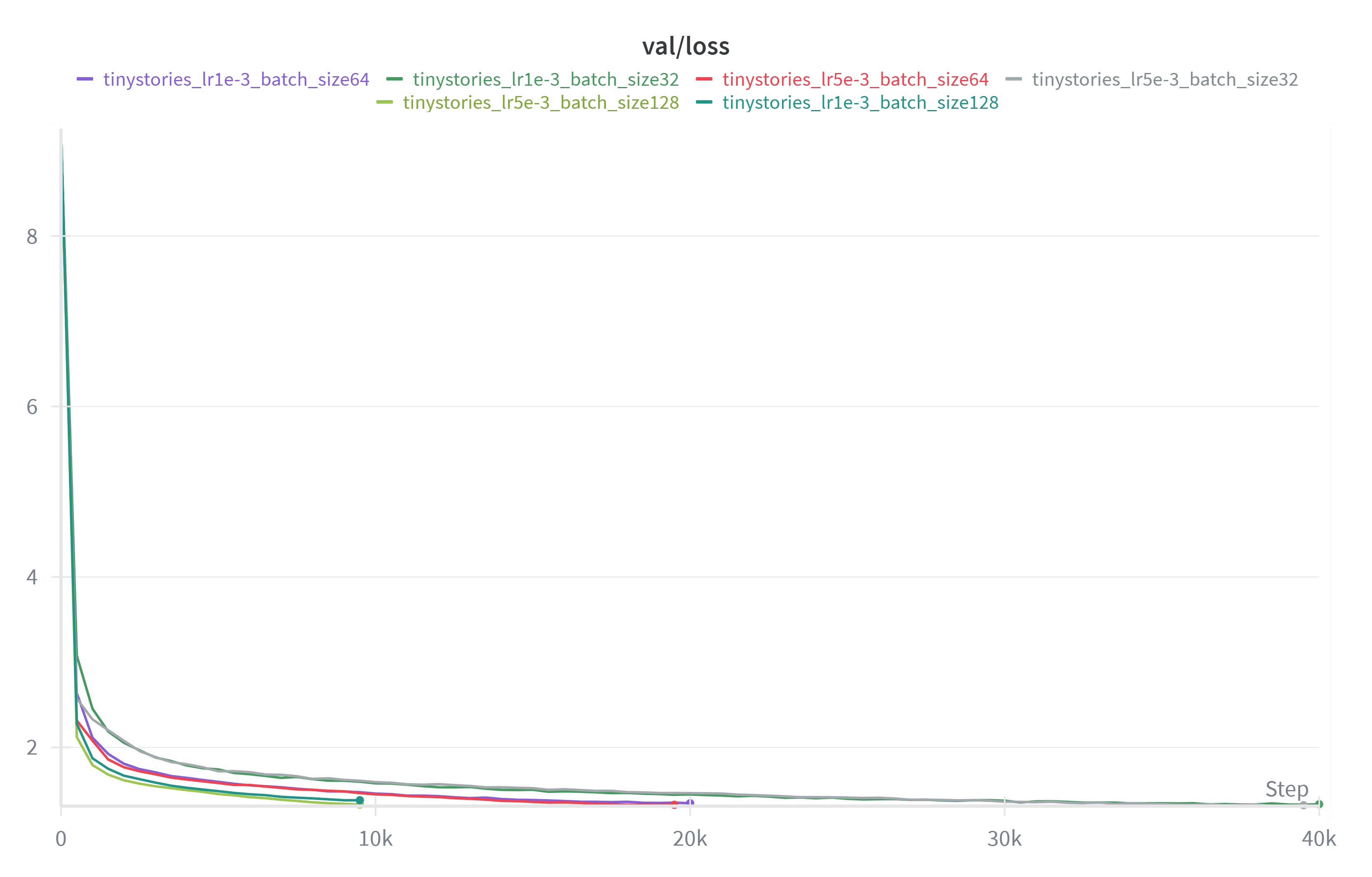
这是我对于 lr 进行的尝试。发现当 lr 为 1e-4 的时候收敛速度就相当慢，而 lr 为 1e-3 的时候最后收敛效果是最好的，validation loss 能降至 1.33 以下（低于 1.45 的 baseline）当 lr 为 5e-4 的时候收敛效果就没那么好了，而当 lr 取 1e-2 的时候训练直接发散。

(b)

发现甚至在 lr=9e-3 的时候表现都较为良好，但一到 1e-2 就发散了。

batch_size

由于要确保总 token 数一样，所以不同的 bs 对应不同的训练步数。在 32 到 128 范围内改变 batch_size 并未对实验结果产生较大影响，不过 bs 取 32 的时候训练时间会略长。

layer_norm_ablation

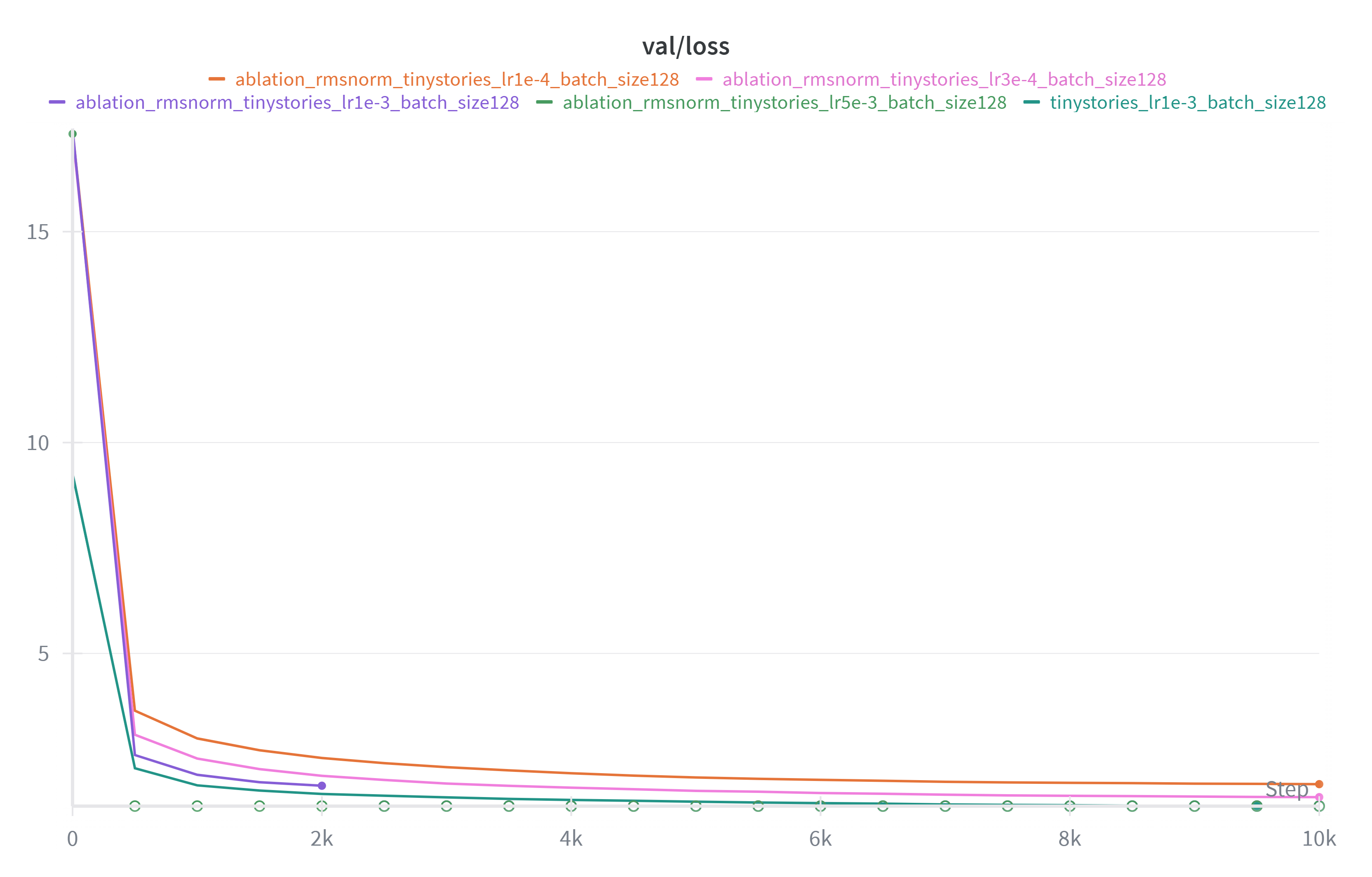
去掉 RMSNorm 后注意到对于 lr=1e-3 和 5e-3 的情况 loss 均在训练一段时间后变为 NaN。未变为 NaN 的情况训练出来效果也显著差。RMSNorm 对保持训练稳定非常重要。

pre_norm_ablation

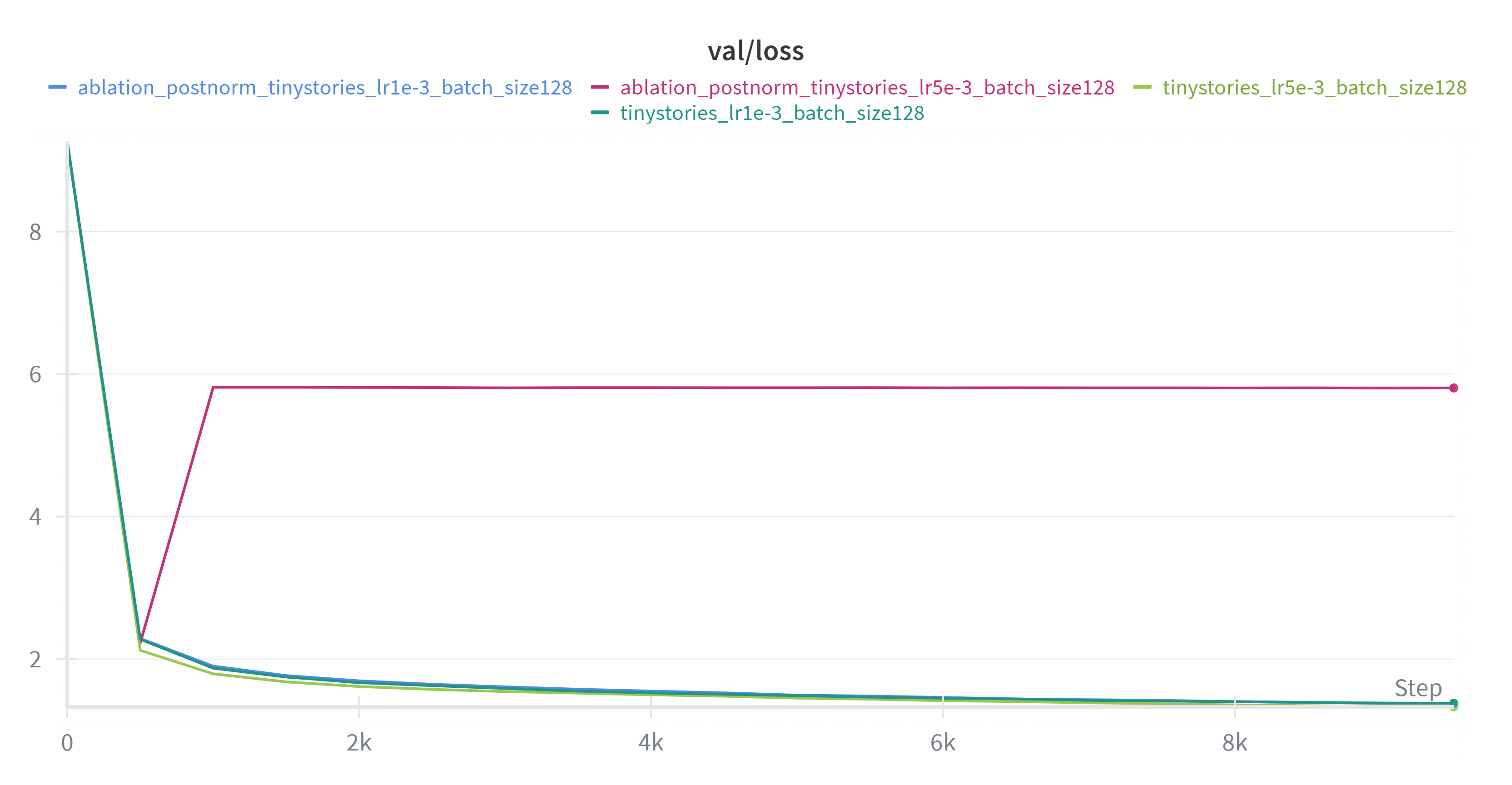
Post norm 稳定性也会变差。

no_pos_emb

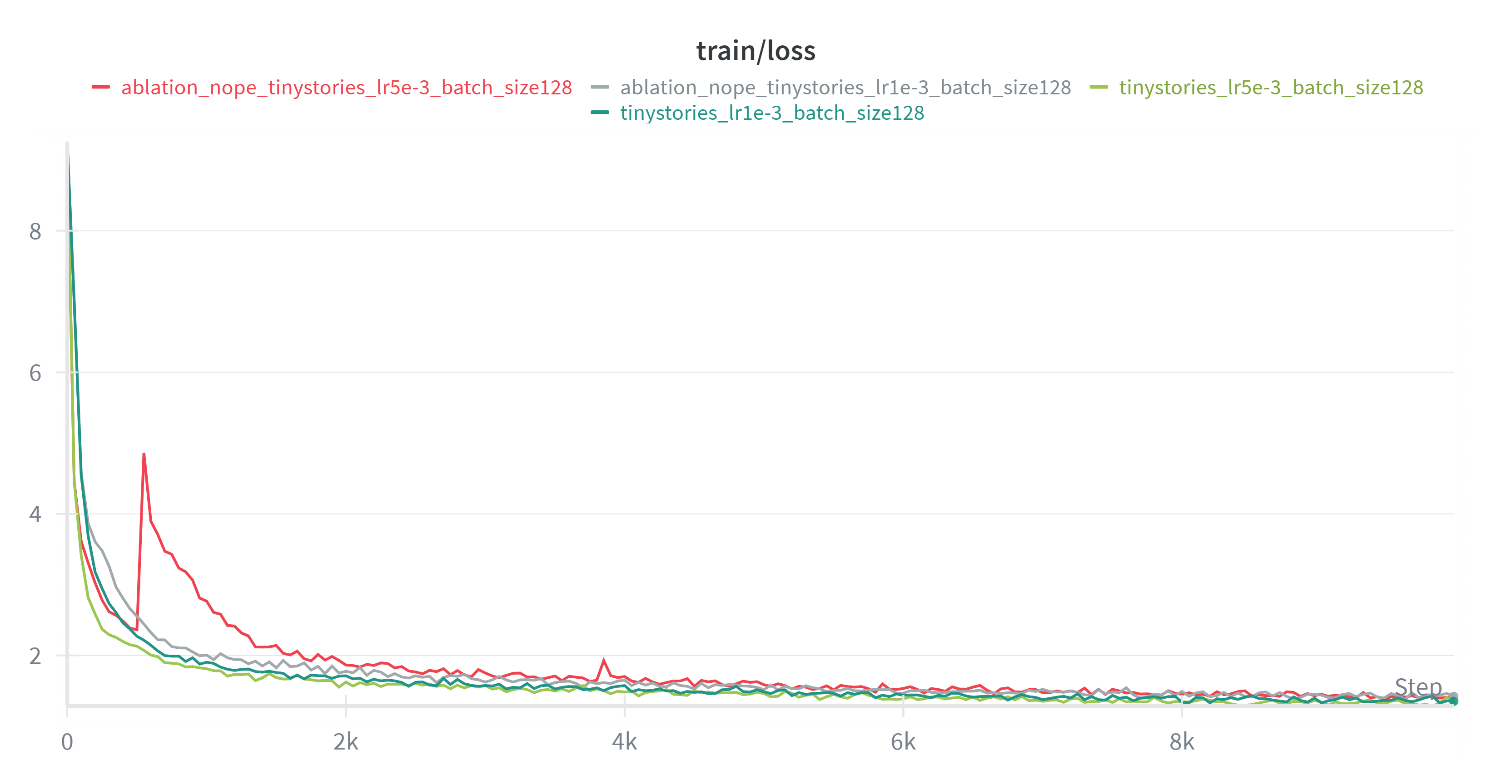
nope 在学习率高的时候可能不太稳定，且效果略差于 RoPE。差距不明显可能源于数据集和模型都比较小。

swiglu_ablation

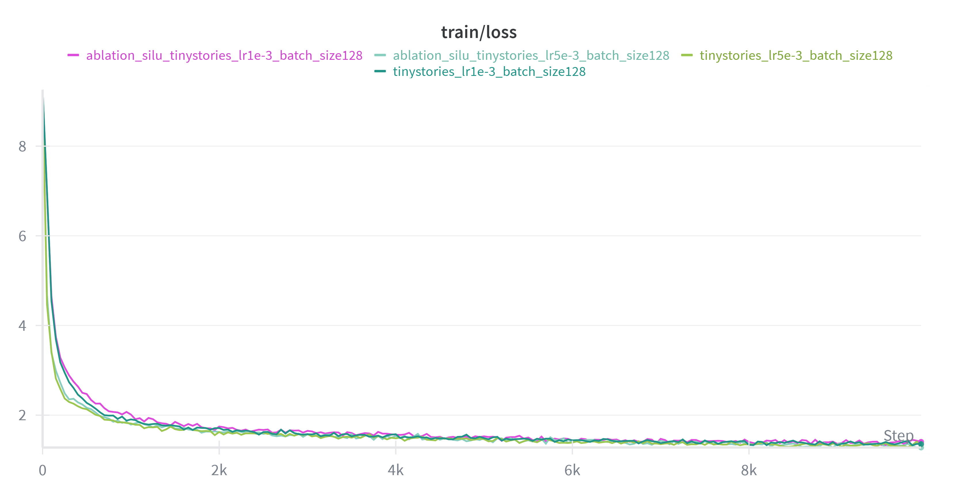
将 SwiGLU 换成 SiLU 后，收敛速度较慢。

main_experiment

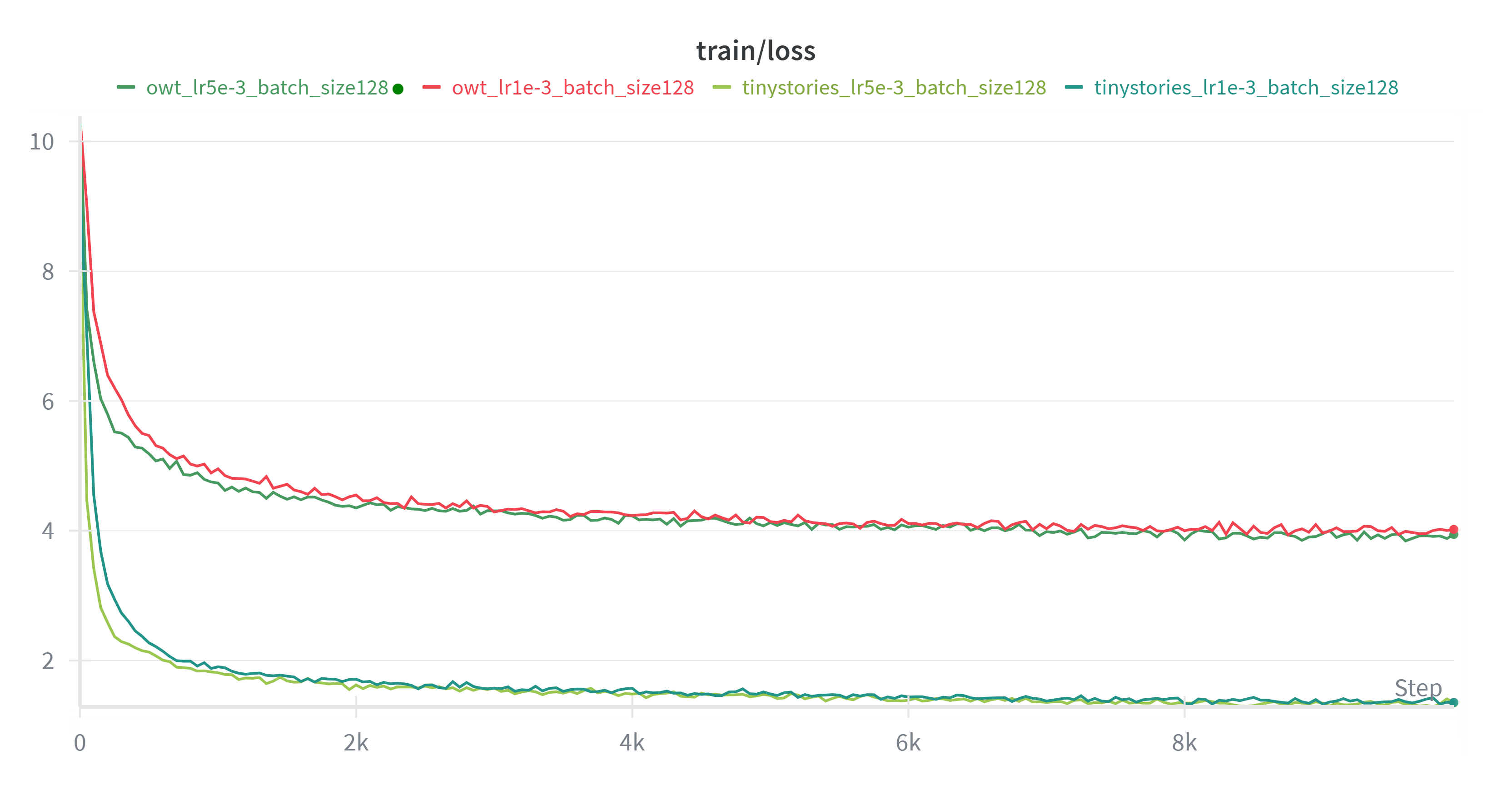
owt 上训的模型 loss 显著高于 TinyStories 上训的模型，因为后者的文本结构简单，可预测性高，而前者覆盖领域广，语言复杂， 条件熵更大，所以 loss 更高。

例子（owt）：Generate a story: Now: func () { public function test.getPost(): You could use the UDP tool (application).getPost(): getPost(): ActivateAgent() protected instrument the Public response to public pronouncements. getPost(): getPost() aView specified { public inquiry into this. see

例子（ts）：Generate a story: a prince was playing with her and her friends. It was a weird story! She had never heard a story before, so she never saw it before. She ran to her mom and asked, "Mom, can I bend down and be Tim?" Mom smiled and said, "You have to be careful when you

因为 TinyStories 的文本分布简单且高度集中，小模型在相同算力下就能学到稳定的叙事结构；而 owt 含有各种各样杂乱的文本，所以在同样训练规模下未能学习到有效模式，因此生成不流畅，质量差。